Autopsie · Economics of disaster risk
Haiti and the Next Major Earthquake: The Cost We Can Already Measure
An economic and financial reading of seismic risk
First published in Le Nouvelliste on 28 August 2026. Read on lenouvelliste.com ↗
Translated from the French original. In case of discrepancy, the French text prevails. Read the French original
The next major earthquake in Haiti cannot be predicted. What can already be done is to put bounds on its economic cost, compare that cost with the country’s means, and measure what would be available to finance the first weeks of reconstruction.
The next major earthquake in Haiti cannot be predicted. Neither its date, nor its epicenter, nor its magnitude can be reliably announced in advance. What can already be done is to put bounds on its economic cost, compare that cost with the country’s means, and, above all, measure what would be available to finance the first weeks of reconstruction.
That is the question this article addresses. In the public sources gathered here, I found no single figure linking, for 2026, potential losses, the state’s financial capacity, and the financing actually pre-arranged. The aim, then, is not to claim to know the bill for the next earthquake down to the last decimal. It is more modest: to put the existing data on a common scale and answer three simple questions. How much could we lose? What share of that loss could fall to the state? And how much money could already be mobilized before outside aid even arrives?
From earthquake to economic risk
To understand the problem, one must distinguish the natural phenomenon from the economic risk it creates. A simple representation rests on four elements: hazard, exposure, vulnerability, and absorptive capacity.
Hazard is the probability that ground motion of a given intensity will occur. Exposure refers to what is on the ground: housing, schools, businesses, roads, ports, bank deposits, or loans. Vulnerability indicates the share of these assets that could be destroyed. Finally, absorptive capacity covers the financial and institutional means of withstanding the shock and getting going again.
The distinction matters because a government does not control the geological fault. It can, however, act on the other three dimensions: limit exposure through land-use planning, reduce vulnerability through building codes that are actually enforced, and prepare in advance the financial instruments that will pay for the first expenditures.
To move from these notions to a financial order of magnitude, let us look at the World Bank’s study. Its 2017 Haiti Country Disaster Risk Profile, taken up in 2019 in the Strengthening Disaster Risk Management and Climate Resilience project, estimates potential losses at several levels of rarity. To represent an extreme shock, it uses, among others, a “250-year return period.”
Where does the “250-year” benchmark come from?
The number 250 does not come from the time elapsed between two Haitian earthquakes. It comes from the risk model. The model combines many plausible earthquakes, the intensity of the shaking they would produce, the exposed assets, and their vulnerability. It thus obtains a range of losses, from the most frequent to the most exceptional.
These losses are ranked by their probability of being exceeded in a given year. The “250-year” benchmark corresponds to an annual probability of 1 in 250, or 0.4%. That is where the number comes from: 1 / 0.004 = 250. The World Bank specifies that this threshold serves to represent an extreme event.
So this does not mean that such an earthquake occurs exactly every 250 years, or that Haiti has 250 years ahead of it. With a constant annual probability of 0.4%, the cumulative risk reaches about 11.3% over thirty years and 18.2% over fifty years. Rare, then, does not mean negligible on the scale of a building or a mortgage.
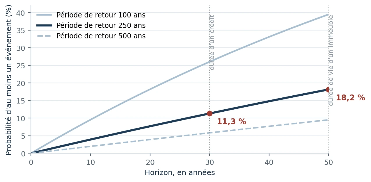
This is the benchmark that the Haiti Country Disaster Risk Profile uses to put a figure on extreme seismic risk. The result cited by the World Bank in 2019 is a probable maximum loss of $2.41 billion, or 27.5% of 2016 GDP. It is neither the predicted cost of a future earthquake nor an earthquake of a specific magnitude: it is a modeled level of loss associated with this threshold of rarity. The 2019 source refers explicitly to the World Bank’s 2017 Haiti Country Disaster Risk Profile.
The reference point, then, is indeed 2016. In the rest of this article, applying the 27.5% ratio to 2026 GDP serves only to construct a stress scenario of comparable size. It does not update the World Bank’s seismic model, and it does not turn $10.77 billion into a forecast.
Two risks, two financial logics
Haiti has to manage two very different profiles. Hurricanes and floods recur frequently and erode capital through repeated small and medium-sized losses. Major earthquakes are much rarer, but their cost can become systemic. This difference explains why they are not financed in the same way.
The 2014 diagnostic by the World Bank and the Ministry of Economy and Finance (MEF) put the average annual loss at $118 million for hurricanes and $26 million for earthquakes. These amounts are annualized: they smooth events of differing frequency and severity over a long period. They should not be confused with the $2.41 billion in the 2017 risk profile, which describes an extreme loss associated with the 250-year benchmark. The two estimates come from different modeling exercises and do not form a single statistical series. They answer two distinct questions: how much the risk costs on average over time, and how high a rare shock can go. Over the period 1961–2012, the 2010 earthquake alone accounted for 93% of recorded damage and 91% of deaths.
The following table summarizes the difference that matters for financial policy: frequent losses can be partly absorbed by budget reserves; extreme losses require mechanisms capable of transferring part of the risk before the disaster.
| Characteristic | Frequent risks (hurricanes, floods) | Rare, extreme risks (earthquakes) |
|---|---|---|
| Frequency | High | Low |
| Severity of a single event | Often localized to significant | Potentially systemic |
| Main origin | Hydrometeorological | Seismic |
| Economic effect | Repeated erosion of capital and income | Sudden destruction of a large stock of assets |
| Financial response | Reserves, provisions, reallocations | Insurance, contingent credit, risk transfer |
Table 1 · Two risk profiles that call for different financial responses.
Between April and July 2026, the Technical Seismology Unit of the Bureau of Mines and Energy detected 136 earthquakes, 118 of them of magnitude 3 or less. This activity, described as low to moderate, gives no grounds for announcing that a major event is imminent. It is simply a reminder that seismic risk is a permanent feature of the country’s environment.
The useful question then becomes very concrete: if a major shock struck the Haitian economy as it stands today, what financial order of magnitude should one have in mind?
What would a major earthquake cost today?
There is no single figure valid for every question. Three methods can be used, but they do not measure the same thing. Conflating them creates an illusion of precision that the data do not allow.
| Method | What it actually measures | Haitian example | What it does not tell you |
|---|---|---|---|
| Retrospective | Damage and losses actually observed after an event | 2010 earthquake: $7.8 billion, or 117% of GDP at the time | Nothing about current exposure |
| Probabilistic | A modeled loss associated with a probability level | World Bank: probable maximum loss of $2.41 billion, or 27.5% of 2016 GDP | Exactly what an earthquake would cost in 2026 |
| Conventional | A fiscal stress-test assumption | Fiscal stress: shock calibrated at 25% of GDP | A physical estimate of destruction |
Table 2 · Three methods, three different questions.
First reading: update the 2010 bill. Damage and losses had been assessed at about $7.8 billion. Adjusting for US inflation alone between 2010 and 2026 gives about $11.95 billion. This calculation takes no account of new buildings, population movements, or the transformation of the economy. It is a monetary equivalent, not a physical estimate of what would be destroyed today.
Second reading: use the World Bank’s benchmark for the 250-year return-period earthquake. The published figure is a probable maximum loss of $2.41 billion, or 27.5% of 2016 GDP. Applying the same ratio mechanically to the IMF’s projection of nominal GDP for 2026 gives $10.77 billion. This transposition serves only as a fiscal stress of comparable size: it does not update the seismic model and is not an estimate of what would be physically destroyed in 2026.
Third reading: reason from the macroeconomic scale actually observed in 2010. The 2014 diagnostic puts the earthquake’s damage and losses at around 117% of GDP at the time. As a stress scenario, a shock equivalent to 100% or 120% of 2026 GDP would represent about $39 billion to $47 billion. But the 117% of 2010 and the 27.5% of the probabilistic model are not directly comparable: the first figure is an ex post assessment of the damage and losses caused by an actual event; the second is an ex ante modeled loss associated with a probability level. They are used here as benchmarks of scale, not as results of the same method.
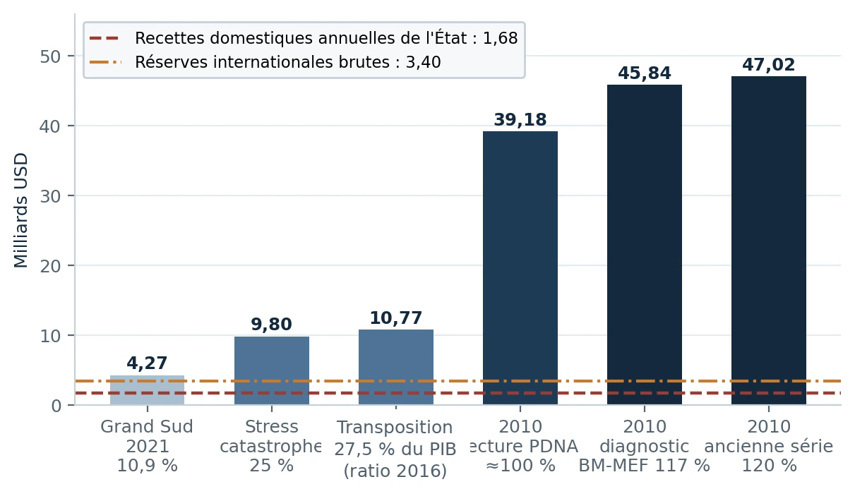
These approaches therefore yield very different amounts because they answer different questions. That is precisely why caution is in order. The only robust figure at this stage is not “the cost of the next earthquake,” but the scale of the financial vulnerability that a major shock would expose.
To see this, let us compare these losses with the state’s ordinary means. The IMF projects domestic revenue for 2026 at 4.3% of GDP, or about $1.68 billion. Each scenario can then be converted into a number of years of domestic revenue.
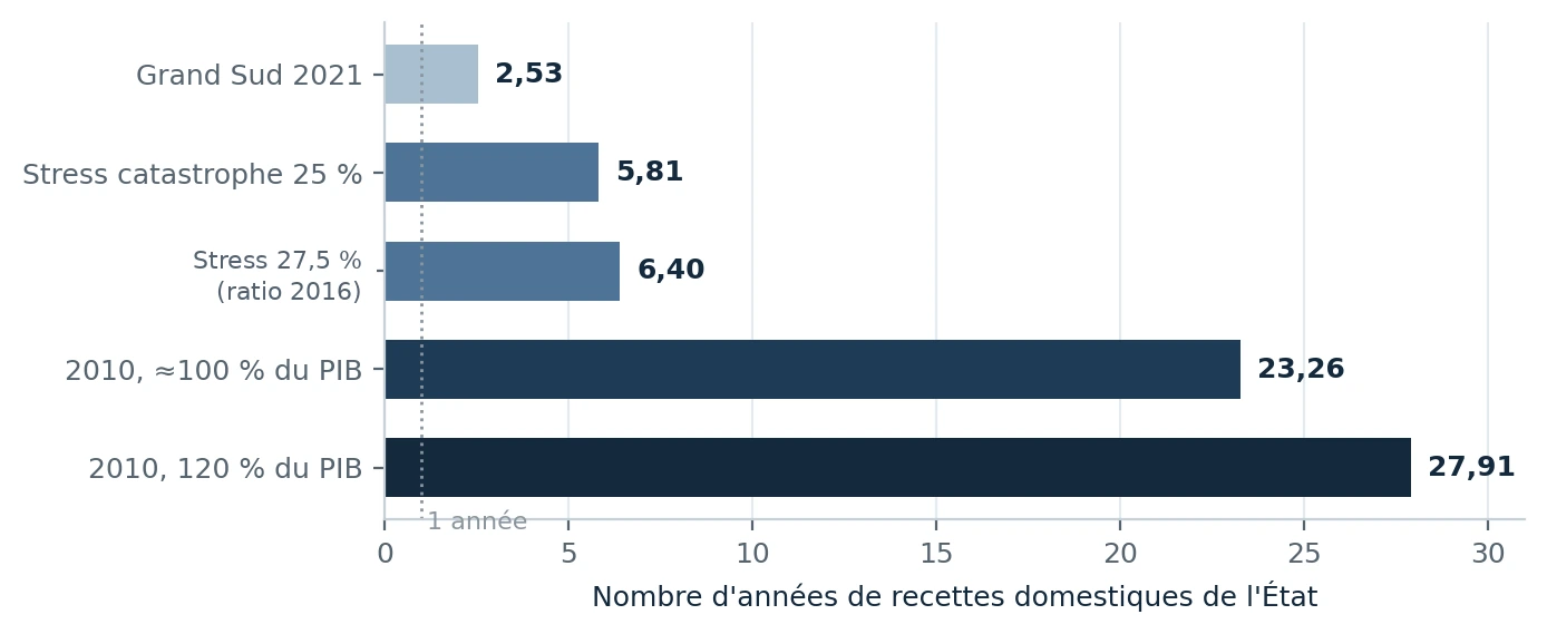
A shock of 25% of GDP represents about 5.8 years of domestic revenue; the stress equivalent to 27.5% of GDP, 6.4 years; a shock equal to 100% of GDP, more than 23 years. These comparisons do not indicate how long reconstruction would actually take. They simply show that a large shock would far exceed what current revenue can absorb on its own.
This fiscal weakness is at the heart of the problem. It means that preparedness cannot rest solely on the idea that the budget will be reallocated after the disaster. Part of the financing must be arranged before the shock.
Nor are the international reserves of the Bank of the Republic of Haiti (BRH), the central bank, projected at around $3.4 billion at the end of 2026, an insurance fund. They support external liquidity and the capacity to pay for imports. Yet a major reconstruction increases precisely the need for imported medicines, fuel, steel, cement, and equipment.
The constraint is therefore twofold: after a major earthquake, budgetary resources must be found for reconstruction while preserving the foreign exchange the economy needs to function. This tension explains why the question of financing must be raised before the disaster.
The shock does not stop at buildings
An economic catastrophe is not just the houses, schools, or roads that collapse. The 2010 earthquake shows very concretely what happens after the first tremor. The Post-Disaster Needs Assessment (PDNA) separated damage, that is, the value of the buildings, equipment, and infrastructure destroyed, from losses, that is, the activity that no longer takes place afterward: interrupted production, lost sales, vanished wages, additional costs. Of the $7.8 billion in effects estimated in 2010, about 55% was physical destruction and 45% was these flow losses. In other words, nearly one dollar in two on the bill already had nothing to do with a wall to be rebuilt.
The distinction is even sharper in the productive sectors. There, the PDNA estimated $302 million in physical damage but $934 million in lost activity: three-quarters of the economic effect thus came from what was no longer produced, sold, or earned after the earthquake.
| Sector | Physical damage (USD million) | Activity losses (USD million) | Losses / damage |
|---|---|---|---|
| Industry | 75 | 268 | 3.6× |
| Commerce | 149 | 491 | 3.3× |
| Total (4 sectors) | 302 | 934 | 3.1× |
Table 3 · In 2010, activity losses far exceeded physical damage in the productive sectors. The total also includes agriculture and tourism. Source: PDNA Haiti 2010, Productive Sectors Working Group. Amounts rounded.
The table tells the story of how the shock spread better than any formula could. In industry, about $75 million in assets had been damaged, but activity losses reached $268 million, more than three times that amount. In commerce, $149 million in physical damage came with $491 million in losses. A business can therefore remain standing and still lose several months of activity because its suppliers no longer deliver, electricity is lacking, roads are cut, or its customers have themselves lost their income.
The chain is fairly simple. An unusable road or port delays goods; a business cuts production; employees work less or lose their jobs; households consume less; tax revenue falls at the very moment the state must finance relief. After the 2010 earthquake, the World Bank thus estimated that projected government revenue for fiscal year 2009–2010 had fallen by about 20%, under the combined effect of the contraction in activity and the damage suffered by the tax administration. The physical shock had already turned into a fiscal shock.
Reconstruction adds one last strain: it increases the need for imported fuel, steel, cement, medicines, and equipment precisely when the economy and the public finances are weakened. There is no need to assign this propagation an artificially precise multiplier to grasp what it means: the rubble is only the first line of the bill. The next lines hit incomes, the state, and finally credit. It is this last channel that makes the concentration of banking in the Ouest department particularly important.
Banking risk: a concentration hard to ignore
The financial system adds another dimension to the problem. Diversification protects a loan portfolio when borrowers’ difficulties do not all arise in the same place at the same time. A major earthquake in the metropolitan region, by contrast, creates a common shock: premises destroyed, real-estate collateral damaged, activity interrupted, and household incomes hit, all at once.
The question, then, is not only how many loans have been made, but how geographically concentrated they are.
As of 31 March 2026, the Credit Information Bureau (BIC) recorded about 239.30 billion gourdes in outstanding loans, 75.81% of them in the Ouest department. This proportion alone is enough to show that territorial risk is highly concentrated.
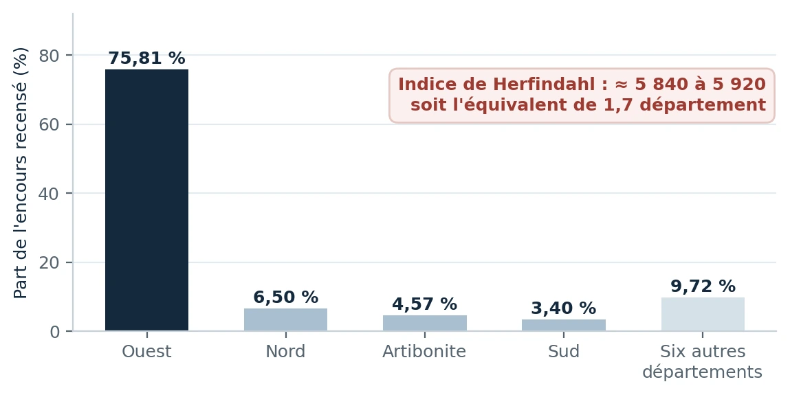
A Herfindahl index applied to this distribution comes out at around 5,900, depending on how the six departments grouped together in the remainder are allocated. The figure serves only to summarize concentration: the thresholds used in competition law should not be applied to it mechanically.
To give an order of magnitude, the BIC’s outstanding loans in the Ouest, about 181.41 billion gourdes, can be subjected to a few stress assumptions. The table below does not attempt to forecast defaults after an earthquake. It only shows how the loss varies as the share of outstanding loans put under stress and the final loss on those loans increase.
| Scenario | Ouest loans under stress | Final loss on those loans | Estimated loss (HTG billion) |
|---|---|---|---|
| Moderate | 20 % | 20 % | 7,26 |
| Intermediate | 30 % | 35 % | 19,05 |
| Extreme sensitivity case | 40 % | 50 % | 36,28 |
Table 4 · Three sensitivity scenarios applied to the BIC’s outstanding loans in the Ouest. This is an illustrative exercise, not a prudential projection.
In the intermediate scenario, 30% of outstanding loans would come under stress and 35% of that exposure would ultimately be lost, about 19.05 billion gourdes. In the extreme sensitivity scenario, the loss would reach 36.28 billion. These amounts should not be compared directly with the banking system’s published capital without reconciling statistical coverage: the BIC’s universe and that of the banks’ balance sheets are not the same.
What the Jamaican example shows
No state can finance every possible loss on its own. Modern strategies therefore spread the risk in layers: the budget absorbs small expenditures, a contingent credit line provides liquidity quickly, parametric insurance covers a higher tranche, and, for extreme events, a catastrophe bond can transfer part of the risk to financial markets.
The point of this architecture is not to eliminate disaster. It is to know, before disaster strikes, which instrument will pay for which tranche of loss and how fast the money can be mobilized.
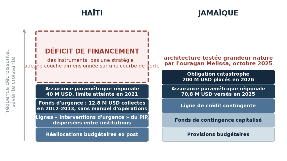
Jamaica offers a concrete regional example. After Hurricane Melissa in 2025, CCRIF paid out $70.8 million. A catastrophe bond provided an additional $150 million without creating new debt at the moment of the shock. In May 2026, the country issued a new $200 million catastrophe bond.
This does not mean that the Jamaican model can be copied mechanically in Haiti. Fiscal capacity, markets, and institutions differ. But the principle is transferable: a rare disaster must be prepared for as a financing problem, with layers identified in advance.
Haiti already has some instruments, notably CCRIF coverage and emergency budget mechanisms. What the public sources gathered here do not make clear is how they currently fit together, what limits remain available, and the total amount that could actually be mobilized after a major earthquake. The problem, then, is not necessarily the absence of any instrument; it is the absence of a consolidated, legible architecture.
This distinction matters. Before proposing a new instrument, one would first need to know what actually exists, under what conditions it can be triggered, and what fraction of the need it covers.
This is where the analysis meets public governance: the best financial strategy begins with a reliable inventory.
The key figure: the financing gap
To estimate post-disaster needs correctly, one must know the exposed assets, their vulnerability, the possible interruptions of activity, and the share that would fall to the public sector. In the public sources examined here, Haiti does not yet have a consolidated inventory that would allow this equation to be closed with precision.
Yet the most useful figure is not necessarily the total loss. It is the gap between that loss and the money already secured before the shock. That gap is the financing gap.
In this definition, pre-arranged financing must be understood in the strict sense: reserves actually earmarked, a signed contingent credit line, insurance limits in force, or any other contractually available mechanism. Ordinary tax revenue should not be treated as a catastrophe fund, since it already finances the day-to-day running of the state.
In the absence of a consolidated public inventory of these resources for 2026, it would be misleading to publish a net gap here as if it were known. One can, however, calculate the gross needs associated with several conventions. On a stress of 25% of GDP, direct public damage would amount to about $2.65 billion if 27% is used; the 70% working assumption used in the 2014 diagnostic leads to $6.86 billion. The 156% ratio observed for the cost of the post-2010 reconstruction program gives $15.29 billion, but it measures something else: a reconstruction program can exceed the value of direct public damage.
| Assumption / convention | Gross need (USD billion) | What the figure measures |
|---|---|---|
| Direct public damage: 27% | 2,65 | Physical share attributed to the public sector |
| Working assumption: 70% | 6,86 | Broader public burden used in the diagnostic |
| 2010 reconstruction program: 156% | 15,29 | Historical cost of the program, not the direct share of public damage |
Table 5 · Gross needs associated with the stress of 25% of GDP. These amounts are not net financing gaps.
Above all, this table shows why the definition of need must be explicit. Depending on whether one is talking about destroyed public assets alone, a broader public burden, or the cost of a reconstruction program, the amount changes sharply. Before seeking further precision, there must first be agreement on what is being measured.
The underlying problem can now be stated without any complicated equation: Haiti has high seismic exposure, concentrates a large share of its credit and activity in the Ouest, has domestic revenue that is small relative to an extreme shock, and does not yet publish a consolidated inventory of pre-arranged financing. The risk is not only of losing a great deal; it is of having to look for the money after the loss.
The aim of this exercise, then, is not to say that the next earthquake will cost $10 billion, $12 billion, $40 billion, or $47 billion. The available data do not allow such certainty. What they do allow is to show that the orders of magnitude can very quickly exceed the country’s fiscal capacity, and that one figure is still missing: how much would actually be available in the first hours, the first months, and the first years?
Methodological note
The calculations presented here should be read as orders of magnitude. The 27.5% ratio corresponds to a probable maximum loss modeled by the World Bank and expressed relative to 2016 GDP; its transposition to 2026 GDP is merely an equivalent stress. It should not be equated with the 117% of GDP measured after 2010, which covers the damage and losses observed ex post. Likewise, the average annual losses of $118 million for hurricanes and $26 million for earthquakes come from the 2014 diagnostic, whereas the $2.41 billion benchmark comes from the 2017 risk profile: these estimates shed light on different dimensions of risk and are not combined as a single series. The banking scenarios are based on the BIC’s outstanding loans and do not constitute a prudential projection. Finally, the net financing gap is not calculated, for lack of a consolidated public inventory of the pre-arranged resources currently available.
Sources
Bureau of Mines and Energy, Technical Seismology Unit: monthly seismic bulletins, April to July 2026. · US Geological Survey, “Can you predict earthquakes?”
World Bank and the Directorate of Economic Studies of the Ministry of Economy and Finance, “Diagnostic sur l’impact économique et budgétaire des désastres en Haïti,” team led by Michel Matera, Disaster Risk Management and Reconstruction project (P126346), funded by the European Union under the ACP-EU Natural Disaster Risk Reduction Program administered by the GFDRR, copyright 2014. Historical risk profile and MPRES probabilistic modeling, tables 2 and 3; impact of the 2010 earthquake at 117% of GDP; public share of damage and cost of reconstruction programs, table 4. Reproduction permitted for non-commercial purposes, provided the source is cited.
World Bank, PDNA Haiti 2010: total effects estimated at $7.804 billion; about 55% physical damage and 45% economic flow losses; productive sectors, $302 million in damage and $934 million in losses. · World Bank, press release of 17 August 2010: a drop of about 20% in projected government revenue for fiscal year 2009–2010 after the earthquake.
World Bank, Strengthening Disaster Risk Management and Climate Resilience Project (P165870), Project Appraisal Document, 25 April 2019, p. 7, note 8, citing Haiti Country Disaster Risk Profile, World Bank 2017: probable maximum losses associated with a 250-year return period, estimated for earthquakes at $2.41 billion, or 27.5% of 2016 GDP; note 7 specifies that this benchmark is indicative of an extreme event. · PDNA Haiti 2010.
International Monetary Fund: World Economic Outlook, April 2026, nominal 2026 GDP of $39.18 billion; country report of May 2026, domestic revenue at 4.3% of GDP; press release of 6 April 2026, gross reserves of around $3.4 billion; country report CR 26/107, imports of goods and services. · World Bank and IMF, Debt Sustainability Analysis 2026, conventional catastrophe shock of 25% of GDP.
Bank of the Republic of Haiti: monetary policy note for the second quarter of 2025–2026, bank assets, shareholders’ equity, gross loan portfolio of the banking system, outstanding loans recorded by the Credit Information Bureau and their geographic distribution as of 31 March 2026. · US Bureau of Labor Statistics: consumer price index, 2010 average of 218.056 and July 2026 level of 333.918.
CCRIF SPC: payout of about $40 million to Haiti after the earthquake of 14 August 2021, corresponding to the limit of the 2021–2022 earthquake policy, with the sum insured reinstated for the rest of the policy year under the RSIC; payout of $70.8 million to Jamaica after Hurricane Melissa. · World Bank and Jamaica’s Ministry of Finance: catastrophe bonds of 2021, 2024, and 2026; full $150 million payout triggered by Melissa in October 2025; new $200 million issue in May 2026.